Distributed Order Differential Equations
For more details about distributed order diffeerntial equations and distributed order dynamic systems, we recommend you to read Distributed-Order Dynamic Systems
We integrate ${_0D_t^\alpha f(t)}$ with respect to the order, we can obtain distributed-order differential/integral equations. Since we normally adopted the notation as:
\[{_0D_t^{\omega(\alpha)} f(t)} := \int_{\gamma_1}^{\gamma_2}\omega(\alpha){_0D_t^\alpha f(t)}d\alpha\]
We can write the general form of distributed order differential equations as:
\[\int_0^m \mathscr{A}(r,\ D_*^r u(t))dr = f(t)\]
Similar to what we have learned about single-term and multi-term fractional differential equations in linear fractional differential equations, we can also write the single-term distributed order differential equations:
\[D_*^ru(t)=f(t,\ u(t))\]
And multi-term distributed order differential equations
\[\sum_{i=1}^k \gamma_i D_*^{r_i}u(t) = f(t,\ u(t))\]
Example1: Distributed order relaxation
The distributed order relaxation equation is similar to fractional relaxation equation, only the order is changed to a distributed function. Let's see an example here, the distributed order relaxation:
\[{_0D_t^{\omega(\alpha)} u(t)}+bu(t)=f(t),\quad x(0)=1\]
With a distribution of orders $\alpha$: $\omega(\alpha)=6\alpha(1-\alpha)$
By using the DOMatrixDiscrete method to solve this problem:
The usage of DOMatrixDiscrete method is similar to the FODEMatrixDiscrete method, all we need to do is to pass the parameters array and order array to the problem definition and solve the problem.
Pass the weight function and other orders to the order array in the right way:
julia> orders = [x->x*(1-x), 1.2, 3]
3-element Vector{Any}:
  #3 (generic function with 1 method)
 1.2
 3
using FractionalDiffEq, Plots
h = 0.01; t = collect(h:h:5);
fun(t)=0
prob = DODEProblem([1, 0.1], [x->6*x*(1-x), 0], (0, 1), fun, 1, t)
sol = solve(prob, h, DOMatrixDiscrete())
plot(sol)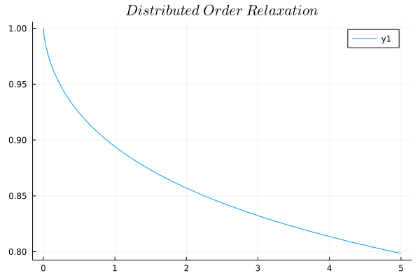
Example2: Distributed order oscillator
When the damping term in Bagley-Torvik equation described by a distributed-order derivative, we get the distributed order oscillator equation:
\[ay''(t)+by^{\omega(\alpha)}(t)+cy(t)=f(t)\]
\[f(t)=\begin{cases} 8, & (0\leq t\leq1)\\ 0, & (t>1) \end{cases}\]
using FractionalDiffEq, Plots
h=0.075; t=collect(0:h:30)
f(t) = 0 ≤ t ≤ 1 ? (return 8) : (return 0)
prob=DODEProblem([1, 1, 1], [2, x->6*x*(1-x), 0], (0, 1), f, [0; 0], t)
sol=solve(prob, h, DOMatrixDiscrete())
plot(sol)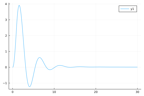
Please see Distributed-Order Dynamic Systems for systematic introduction and knowledge.