Fractional Differences Equations
There are also some solvers can be used to solve Fractional Differences Equations in FractionalDiffEq.jl.
Fractional Differences Equations with the form:
\[\Delta^{\alpha}x(t)=f(t+\alpha,\ x(t+\alpha))\]
With initial condition:
\[x(0)=x0\]
Let's see an example here, we have a fractional differences equation with initial condition:
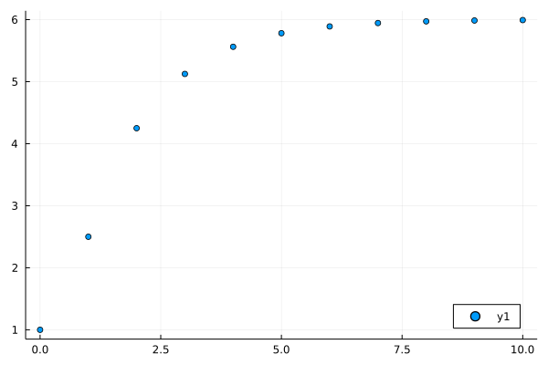
\[\Delta^{0.5}x(t)=0.5x(t+0.5)+1\]
\[x(0)=1\]
By using the PECE solver in FractionalDiffEq.jl:
using FractionalDiffEq, Plots

fun(x) = 0.5*x+1
α=0.5; x0=1;
tspan=(0.0, 1.0); h=0.1
prob = FractionalDiscreteProblem(fun, α, x0, tspan)
sol=solve(prob, h, PECE())
plot(sol, seriestype=:scatter, legend=:bottomright)
And plot the solution:
System of Fractional Difference Equations
Let's see if we have a system of fractional difference equations[1]:
\[\begin{cases} {_3^G\nabla}_k^\alpha x_1(k+1)=-0.05x_2(k)-0.05x_3(k)+0.01\tanh(x_2(k))\\ {_3^G\nabla}_k^\alpha x_2(k+1)=0.05x_1(k)+0.02x_2(k)+0.01\tanh(x_1(k))\\ {_3^G\nabla}_k^\alpha x_3(k+1)=0.1-0.2x_3(k)+0.05x_1(k)x_3(k)+0.01\tanh(x_3(k)) \end{cases}\]
To solve this system of fractional difference equations, we only need to follow the procedure likewise:
using FractionalDiffEq, Plots

function sys!(du, u, p, t)
    du[1] = -0.05*u[2] - 0.05*u[3] + 0.01*tanh(u[2])
    du[2] = 0.05*u[1] + 0.02*u[2] + 0.01*tanh(u[1])
    du[3] = 0.1 - 0.2*u[3] + 0.05*u[1]*u[3] + 0.01*tanh(u[3])
end
prob = FractionalDsicreteSystem(sys!, 0.98, [1, -1, 0])
result = solve(prob, 7, GL())

plot(result[1, :], result[2, :], result[3, :], seriestype=:scatter)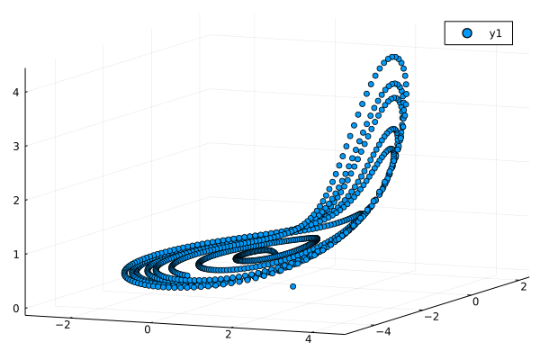
- 1Yiheng Wei, Jinde Cao, Chuang Li, Yang Quan Chen: How to empower Grunwald–Letnikov fractional difference equations with available initial condition?