Fractional Order Delay Differential Equations

In real-world systems, delay is very often encountered in many practical systems, such as automatic control, biology, economics and long transmission lines. The delayed differential equation is used to describe these dynamical systems. Fractional order delay differential equations as the generalization of the delay differential equations, provide more freedom when we describe these systems, let's see how we can use FractionalDiffEq.jl to accelerate the simulation of fractional order delay differential equations.

The fractional delay differential equations have the general form:

\[D^\alpha_ty(t)=f(t,\ y(t),\ y(t-\tau)),\quad t\geq\xi\]

\[y(t)=\phi(t),\quad t\in[\xi-\tau,\ \xi]\]

While only given the initial condition is not enough to solve the delay differential equations, a history function $\phi(t)$ must be provided to describe the history of the system($\phi(t)$ should be a continuous function).

All we need to do is to pass the function $f(t,\ y(t),\ y(t-\tau))$, and history function $\phi(t)$ to the FDDEProblem definition:

prob = FDDEProblem(f, ϕ, α, τ, T)

And choose an algorithm to solve the problem.

Here, we consider the fractional order version of the four-year life cycle of a population of lemmings^[1] (A classical test example for delay differential equations):

\[D^\alpha_ty(t)=3.5y(t)(1-\frac{y(t-0.74)}{19}),\ y(0)=19.00001\]

\[y(t)=19,\ t<0\]

using FractionalDiffEq, Plots
ϕ(x) = x == 0 ? 19.00001 : 19.0
f(t, y, ϕ) = 3.5*y*(1-ϕ/19)
h = 0.05; α = 0.97; τ = 0.8; T = 56
fddeprob = FDDEProblem(f, ϕ, α, τ, T)
V, y = solve(fddeprob, h, DelayPECE())
plot(y, V, xlabel="y(t)", ylabel="y(t-τ)")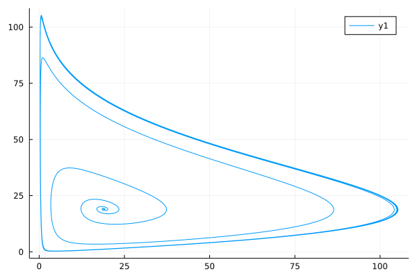

FDDE with multiple lags

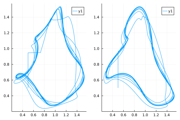
As for FDDE with multiple lags, we need to specify the lag terms by entering the array of lags $\tau$, and call the DelayPECE method to solve the multiple lags FDDE.

\[{_0^CD_t^\alpha}y(t)=\frac{2y(t-2)}{1+y(t-2.6)^{9.65}}-y(t)\\ y(t)=0.5,\ t\leq0\]

using FractionalDiffEq, Plots
α = 0.95; ϕ(x) = 0.5
τ = [2, 2.6]
fun(t, y, ϕ1, ϕ2) = 2*ϕ1/(1+ϕ2^9.65)-y
prob = FDDEProblem(fun, ϕ, α, τ, 100)
delayed, y = solve(prob, 0.01, DelayPECE())

p1=plot(delayed[1, :], y)
p2=plot(delayed[2, :], y)
plot(p1, p2, layout=(1, 2))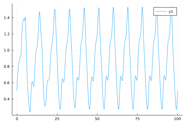

FDDE with variable order

Variable order fractional differential operators give modeling more freedom when we describe the systems. FractionalDiffEq.jl can solve FDDE with variable order derivative no matter single lags or multiple lags. To provide a comprehensive interface, all we need to do is just defining customized FDDEProblem according to our model.

FDDEProblem(f, ϕ, α, τ, tspan)

we can pass α as a Number or a Function to tell FractionalDiffEq.jl it it is a normal constant fractional order FDDE or variable order FDDE.

System of FDDE

Time delay Chen system as a famous chaotic system with time delay, has important applications in many fields. As for the simulation of time delay FDDE system, FractionalDiffEq.jl is also a powerful tool to do the simulation, we would illustrate the usage via code below:

\[\begin{cases} D^{\alpha_1}x=a(y(t)-x(t-\tau))\\ D^{\alpha_2}y=(c-a)x(t-\tau)-x(t)z(t)+cy(t)\\ D^{\alpha_3}z=x(t)y(t)-bz(t-\tau) \end{cases}\]

using FractionalDiffEq, Plots
α=[0.94, 0.94, 0.94]; ϕ=[0.2, 0, 0.5]; τ=0.009; T=1.4; h=0.001
function delaychen!(dy, y, ϕ, t)
	a=35; b=3; c=27
	dy[1] = a*(y[2]-ϕ[1])
	dy[2] = (c-a)*ϕ[1]-y[1]*y[3]+c*y[2]
	dy[3] = y[1]*y[2]-b*ϕ[3]
end
prob = FDDESystem(delaychen!, ϕ, α, τ, T)
sol=solve(prob, h, DelayABM())
plot(sol, title="Fractional Order Chen Delayed System")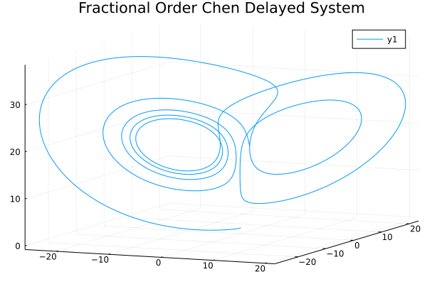

Let's see an detailed example of the fractional order version of enzyme kinetics with an inhibitor molecule:

\[D_t^\alpha y_1(t)=10.5-\frac{y_1(t)}{1+0.0005y_4^3(t-4)}\\ D_t^\alpha y_2(t)=\frac{y_1(t)}{1+0.0005y_4^3(t-4)}-y_2(t)\\ D_t^\alpha y_3(t)=y_2(t)-y_3(t)\\ D_t^\alpha y_4(t)=y_3(t)-0.5y_4(t)\\ y(t)=[60, 10, 10, 20],\ t\leq0\]

using FractionalDiffEq, Plots
function EnzymeKinetics!(dy, y, ϕ, t)
    dy[1] = 10.5-y[1]/(1+0.0005*ϕ[4]^3)
    dy[2] = y[1]/(1+0.0005*ϕ[4]^3)-y[2]
    dy[3] = y[2]-y[3]
    dy[4] = y[3]-0.5*y[4]
end
q = [60, 10, 10, 20]; α = [0.95, 0.95, 0.95, 0.95]
prob = FDDESystem(EnzymeKinetics!, q, α, 4, 150)
sol = solve(prob, DelayABM(), dt=0.01)
plot(sol)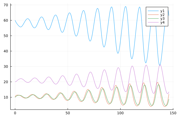

Fractional matrix differential equations with delay

FractionalDiffEq.jl is also capable of solving fractional matrix delay differential equations:

\[D_{t_0}^\alpha\textbf{x}(t)=\textbf{A}(t)\textbf{x}(t)+\textbf{B}(t)\textbf{x}(t-\tau)+\textbf{f}(t)\]

Here $\textbf{x}(t)$ is vector of states of the system, $\textbf{f}(t)$ is a known function of disturbance.

We explain the detailed usage by using an example:

\[ \textbf{x}(t)=\begin{pmatrix} x_{1}(t) \\ x_{2}(t) \\ x_{3}(t) \\ x_{4}(t) \end{pmatrix} \]

\[ \textbf{A}=\begin{pmatrix} 0 & 0 & 1 & 0 \\ 0 & 0 & 0 & 1 \\ 0 & -2 & 0 & 0 \\ -2 & 0 & 0 & 0 \end{pmatrix} \]

\[ \textbf{B}=\begin{pmatrix} 0 & 0 & 0 & 0 \\ 0 & 0 & 0 & 0 \\ -2 & 0 & 0 & 0 \\ 0 & -2 & 0 & 0 \end{pmatrix} \]

With initial condition:

\[\textbf{x}_0(t)=\begin{pmatrix} \sin(t)\cos(t) \\ \sin(t)\cos(t) \\ \cos^2(t)-\sin^2(t) \\ \cos^2(t)-\sin^2(t) \end{pmatrix}\]

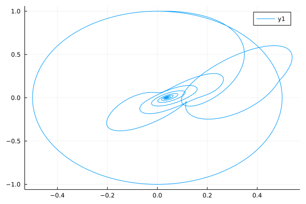
By using the MatrixForm method for FDDE in FractionalDiffEq.jl and plot the phase portrait:

using FractionalDiffEq, Plots

tspan = (0, 70); τ=3.1416; h=0.01; α=0.4
x0(t) = [sin(t)*cos(t); sin(t)*cos(t); cos(t)^2-sin(t)^2; cos(t)^2-sin(t)^2]
A=[0 0 1 0; 0 0 0 1; 0 -2 0 0; -2 0 0 0]
B=[0 0 0 0; 0 0 0 0; -2 0 0 0; 0 -2 0 0]
f=[0; 0; 0; 0]

prob = FDDEMatrixProblem(α, τ, A, B, f, x0, tspan)
sol=solve(prob, h, MatrixForm())
plot(sol[:, 1], sol[:, 3])